Project Summary
Context
This is a transnational data set which contains all the transactions occurring between 01/12/2010 and 09/12/2011 for a UK-based online retail company. The company mainly sells unique all-occasion gifts. Many customers of the company are wholesalers.
The company wants to understand the behavior of their customers over time. They want to know how many of their customers remain active after acquisition. Hence we will run a cohort and retention analysis.
A cohort is a group of persons who have a common trait over an extended period of time. Examples include users who become customers at the same time or a graduating class of students. A cohort analysis can provide a great amount of information for the company and managers as to the behavior of the customers that was acquired or/and converted throughout a campaign. Companies use cohort analysis to understand the trends and patterns of customers over time and to tailor their offers of products and services to the identified cohorts.
Performing a Cohort retention analysis is a useful practice for reducing early customer churn.
Actions
Before running our analysis, we first explored our data. The data contains severals columns which includes the invoice number, stock code, description, quantity, invoice date, unit price, customer id and country. For the purpose of this analysis, we are interested in Invoice date and Customer ID. We dropped all records with missing customer ID and used the Invoice number to filter out all cancelled transactions.
We performed a cohort analysis by grouping the customers into cohorts based on the acquisition time which is the first time they made a purchase. We computed the cohort index which represent the number of months since the acquisitions time and create a cohort table.
We performed the retention analysis by computing the retention rate of each cohort. This is done by dividing the values in cohort table by the corresponding cohort size and converting the resulting values to percentages. We used a heatmap to visualize the result of the retention analysis.
Result
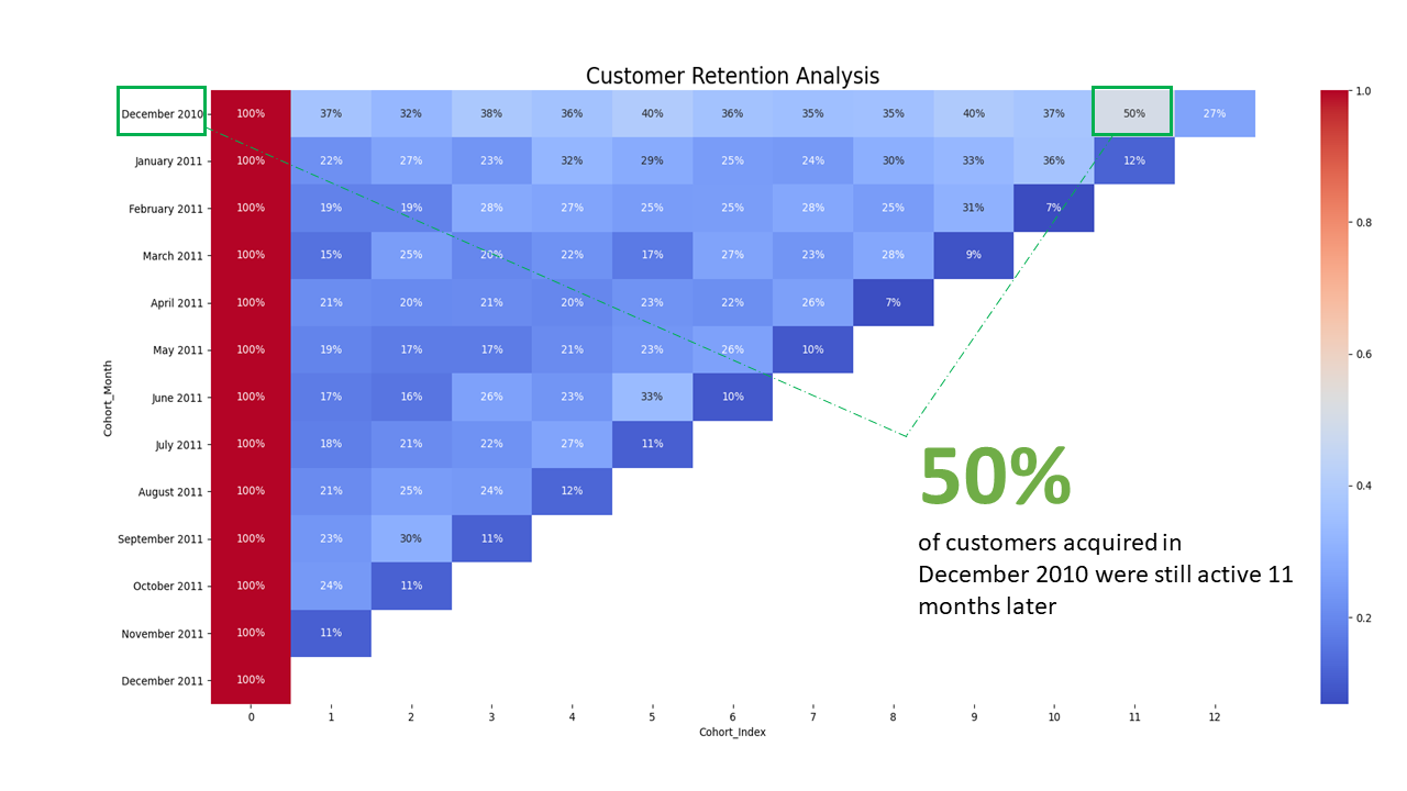
To interpret the result, we have 13 cohorts and 12 cohorts indexes. The retention rate values ranges from 0 to 100% where values closer to 0% bluish, values around 50% are grayish and values closer to 100% are reddish. For instance, the retention rate for December 2010 cohort on the 11th index is 50%. This retention rate means that 50% of the customers that were acquired on December 2010 made a purchase again 11 months later. In other words, 50% of customers acquired in December 2010 were still active 11 months later.
